Human Mobility Prediction
- 15 mins
Even in this age where communication technology is instantaneous, many of us still use or get the response: “If only I knew you are going to be here, I would have…”. This is because people do not constantly update others on where they are heading towards. It is even more so for businesses, as customers rarely keep them informed of their visits. If only businesses know when their customers are arriving or where their customers going, operations can be better optimized, more values can be created for customers and revenues can be improved. Some examples:
- If rental companies know where customers are going to be nearing the end of their rental period, the next potential customer within the vicinity can be offered to take over the vehicle
- If taxi dispatchers know the destinations of rides, customer bookings can be assigned to the driver ending the trip within the vicinity
- If retail stores know that a customer is going to be within the vicinity, tailored promotions can be offered to attract them to the store
- If hospitality businesses know that a customer is going to visit them, they can prepare surprises to uplift customer experience
While explicit information on customer destinations are not available, I am curious to find out if implicit information can be gathered and used to predict customer movement. Nowadays, as almost everyone carries a smartphone by their side most of the time, my hypothesis is:
Destinations of moving objects can be predicted within 3km accuracy if the following data is available:
- Date & Time
- Location data in the form of coordinates via GPS trackers
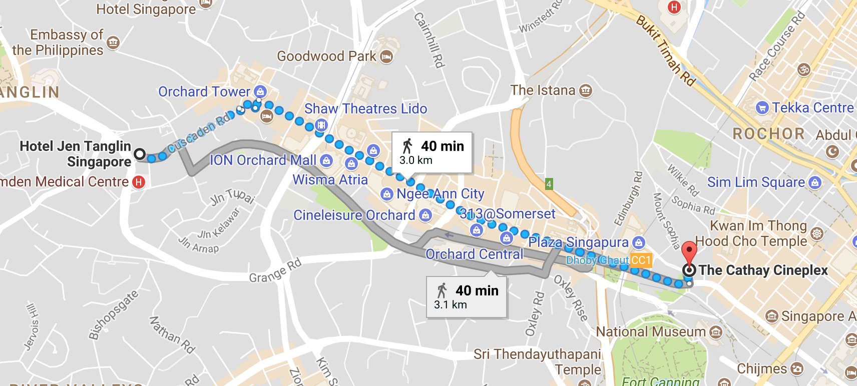
Within 3km accuracy is equivalent to predicting if one is going to be in Orchard, between the Cathy Cineplex to Hotel Jen Tanglin, which is along the busiest retail district in Singapore.
Therefore, for this project, I will explore if my hypothesis is plausible.
For the complete set of Jupyter notebooks with Python code and detailed Markdowns of my process through this project, please refer to my Github.
Data Origin
I am fortunate to be able to gather a year’s worth of taxi trips from the city of Porto from a competition hosted on Kaggle. The objective of the competition is to predict the destination of a taxi ride while the taxi is on the move. Therefore, I have decided to use this to test out my hypothesis on predicting human mobility.
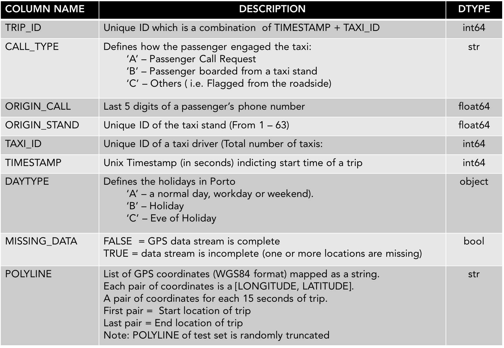
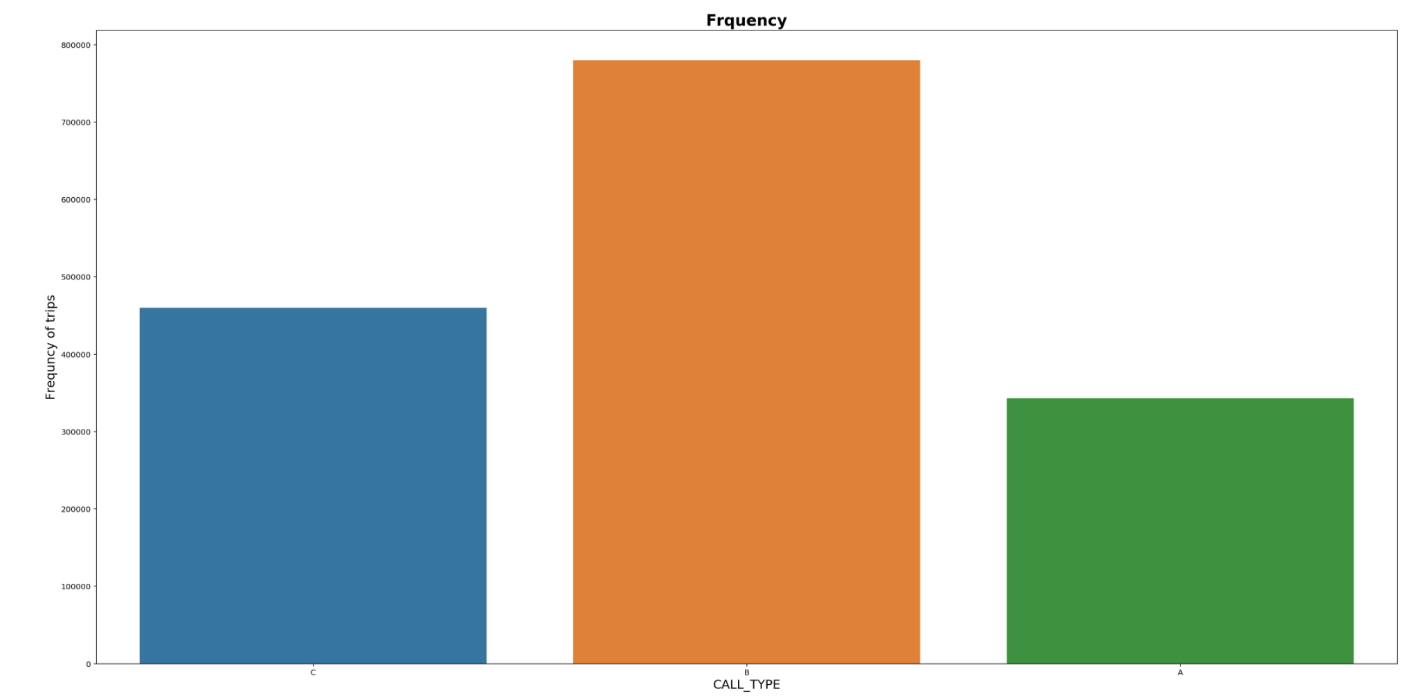
The metadata is as summarize below:
The evaluation method is the Mean Haversine Distance. The Haversine Distance is commonly used in navigation. It measures distances between two points on a sphere based on their latitude and longitude.
The Harversine Distance between the two locations can be computed as follows:
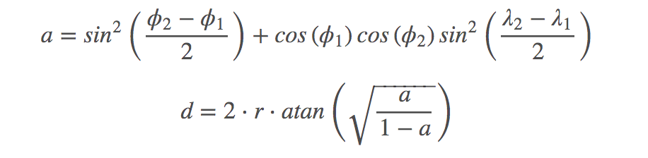
where ϕ is the latitude, λ is the longitude,
d is the distance between two points, and r is the Earth’s radius (6371km).
Approach Taken
- Extract, transform & load (ETL) data onto a VM Instance on Google Cloud
- Perform wrangling and exploratory data analysis (EDA)
- Create Train/Validation datasets
- Create machine learning models using train data
- Regression - Tree Based Models
- Classification – Neural Network
- Validate models using the mean haversine distance and thereafter predict on test data set
ETL
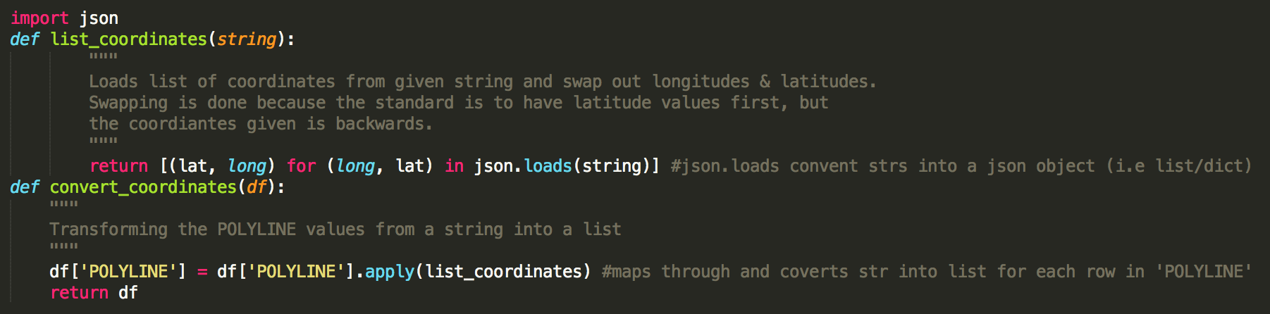
As the dataset consists of over 1.7 million trips, functions are written to efficiently extract, transform and load based on a toy dataset consisting of 50,000 random trips. An interesting point is that “POLYLINE” which contains all the datatype of the GPS coordinates is a string instead of a list, and coordinates (such as start and end coordinates) which is required could not be extracted. Therefore, the “POLYLINE” feature is transformed using the functions written below and the start and end coordinates are extracted.
In addition to transforming the “POLYLINE” feature, duplicates and missing data were also removed. Also, the timestamp data is converted into date and time, with features, quarter hour of a day, day of the week and week of year. After establishing the initial clean processing, these were applied to the main dataset through the use of a virtual machine on Google Cloud.
EDA
With the full dataset that has been initially cleaned, exploratory work can be carried out.
As the predictions is on taxi destinations, all the end points are plotted out to better visualize them.
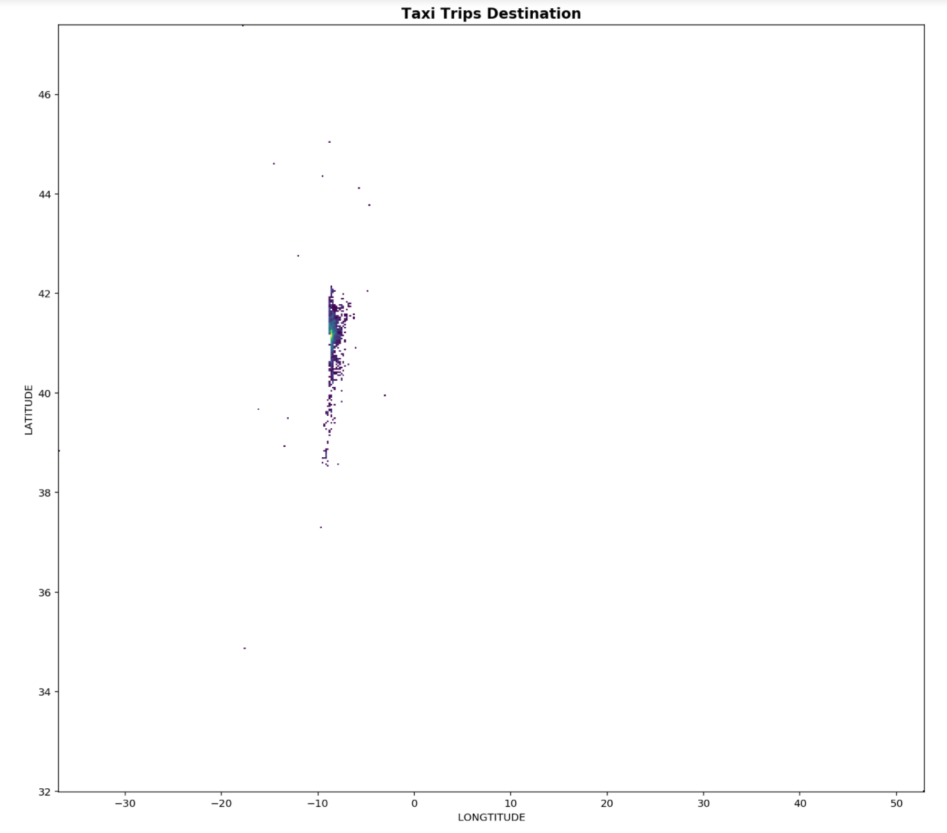
From the plots of the destination coordinates it is observed there are a couple of trips which ended very far away from the majority, are concentrated into a small blob, seen in the figure above. It is important that our training data destinations do not contain end points which are very far away from majority of the end points as this will reduce the accuracy of the model predictions. In order to determine which are the outliers, a statistical approach, using the interquartile ranges of both the latitudes and longitudes are taken.
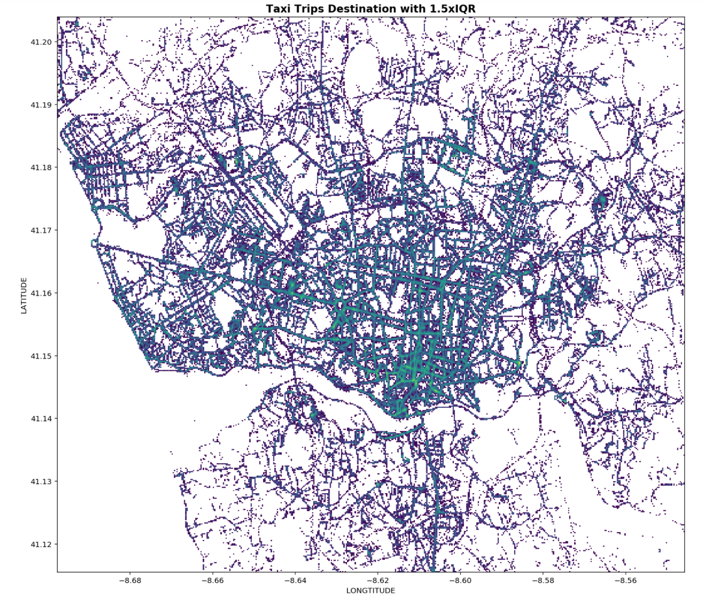
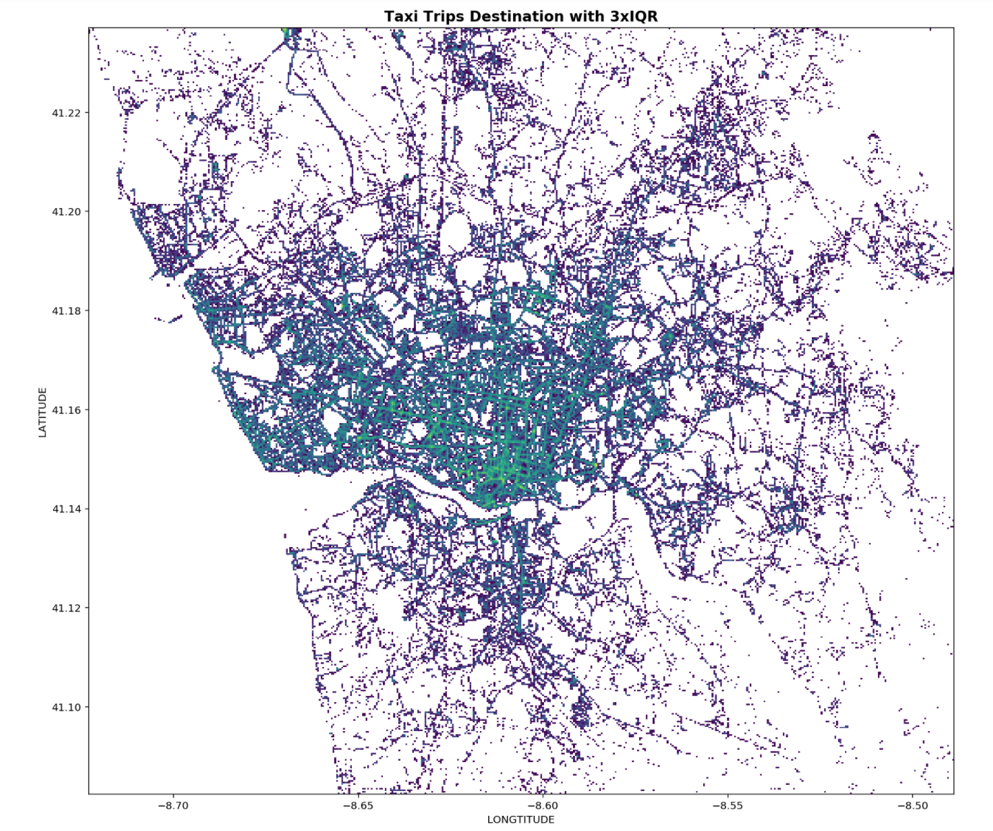
Form the figures above, the points in green are the where most trips end. There is a high concentration of green points which seems to indicate that most trips end at the city centre. The plot with 1.5xIQR seems to a remove a fair bit of popular destinations after comparing the points at the left, top and bottom of both plots. Therefore, 3xIQR is chosen to remove outliers.
Two new features, duration of trips and harversine distance between the start points are engineered with the code below. Trips with NIL duration and NIL distance are removed as that indicated that the taxi is stationary, most like it was due to the driver accidentally activating meter, logging a trip.
Generally distance travelled is proportionally related to duration taken, a scatter is used to visualize this.
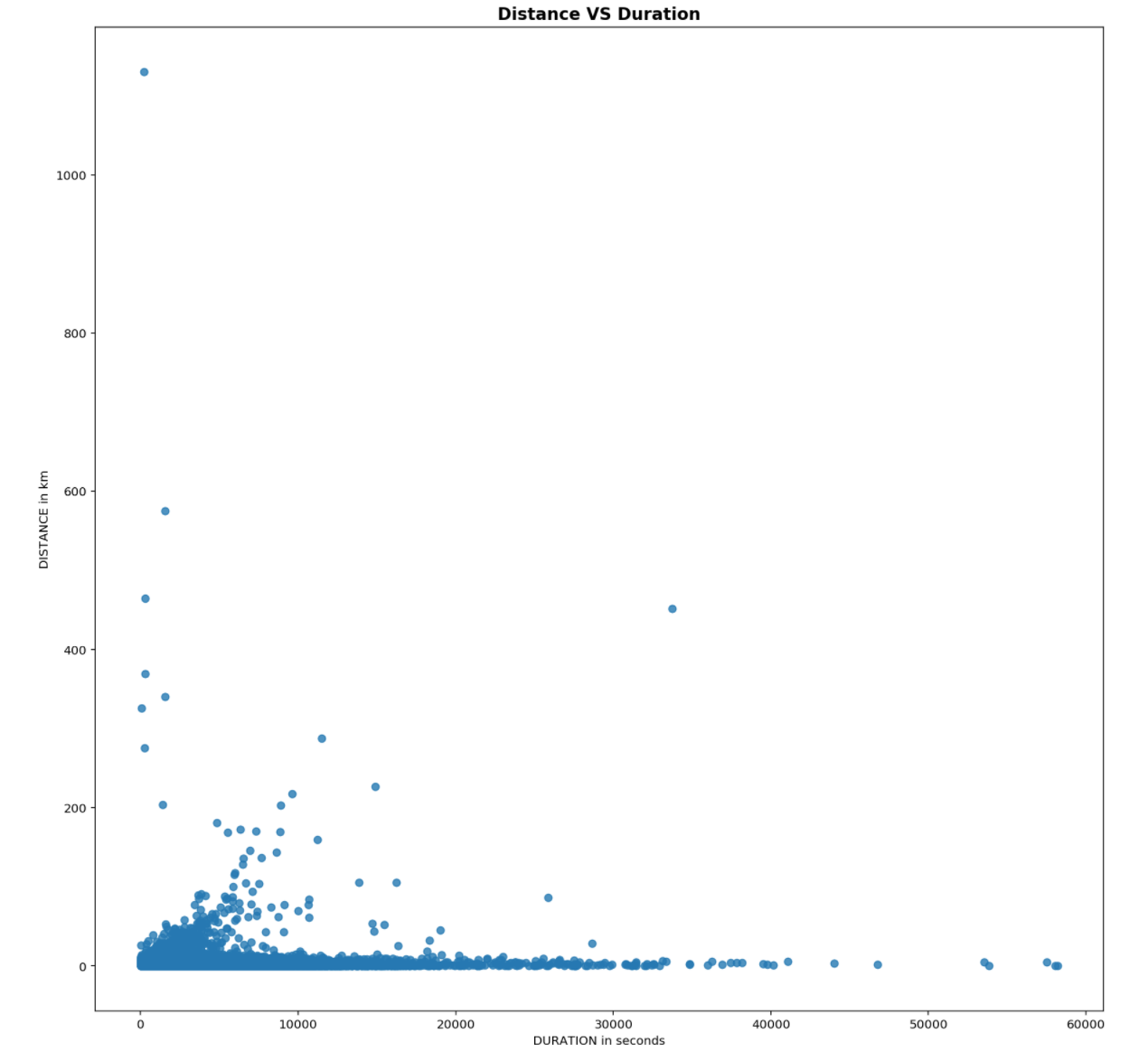
From above, It seems that there is little relationship between both distance and duration. This could be explained as taxis do not travel in a straight path and there are also plenty of turns being made when travelling in a city.
However, on the left hand side of the plot, there are trips which covered a long distance over a short period of time, over 1100km in under 3hours and on the right hand side of the plot, trips which took a long time to complete but only covered a short distance are observed, trips with duration of over 10hours but travelled less than 10km.
In order to removed the noise identified, the same statistical approach using interquartile ranges is utilized. However, as it a noted both distributions of distance and duration are very right skewed, normalization by logging both features is required first.
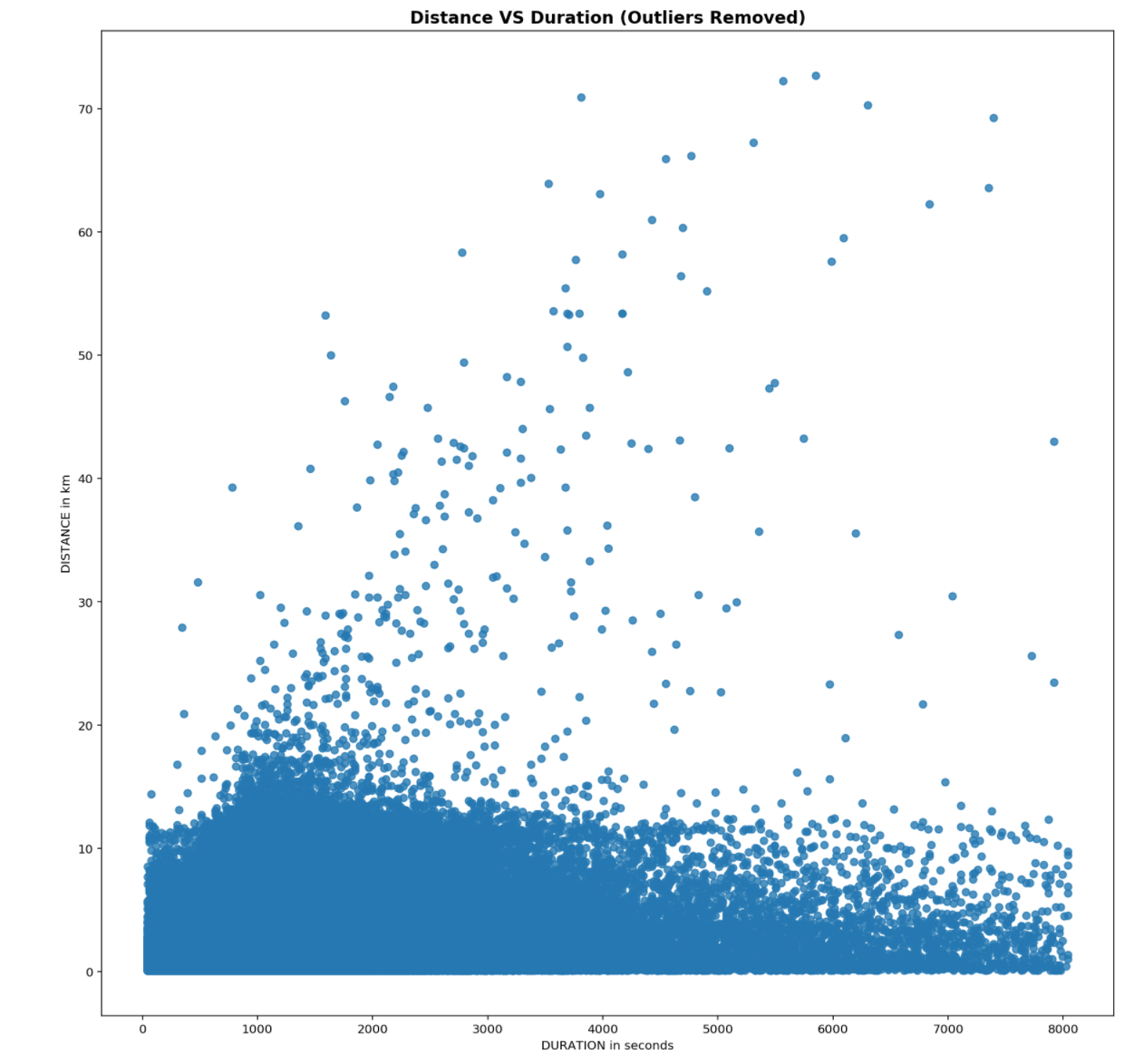
Looking at the both figures above, using 1.5xIQR for trips’ distance and duration will introduce a large amount of bais as the distance of the taxi trips will be range between to 300m - 15km and durations between ~2mins to ~40mins. Whereas by using 3xIQR, the distance of the taxi trips will be range between 0.08 - 60.8km and durations between ~45s to ~2h. Taking into considering the area of end points is ~383km sq, 3xIQR would be a better choice to remove outliers.
At this point, the training dataset is fairly clean. Now, more insights from the taxi trips can be extracted. Using the date and time data extracted, the distribution of the trips can be observed.
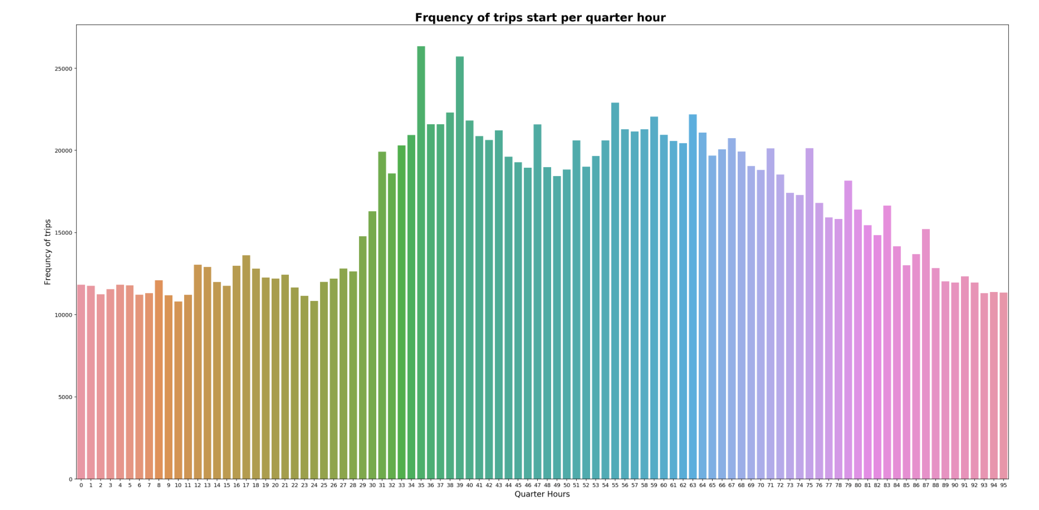
Most taxi rides appear to happen between the day, between 31 - 84 quarter hours, which is ~0800 - 2000 hours. The quarter hour at which most trips are conducted is 35, between 0845 to 0900 might be due to people being late and getting a taxi to rush to work/school. Least trips are conducted at quarter hour 10, between 0230 to 0245.
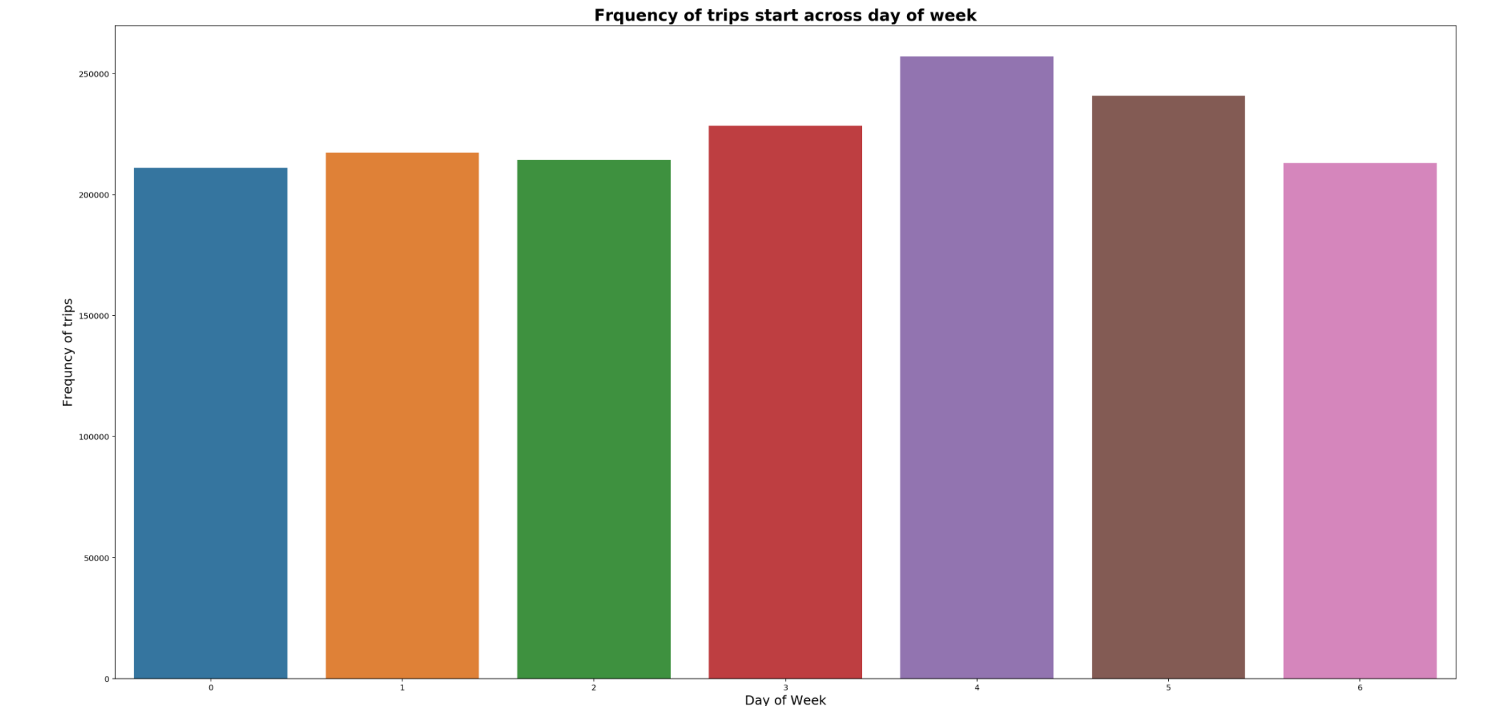
Most taxi trips are on Fridays. It appears that most likely people are out for entertainment to kickstart the weekend and use taxis to commute.
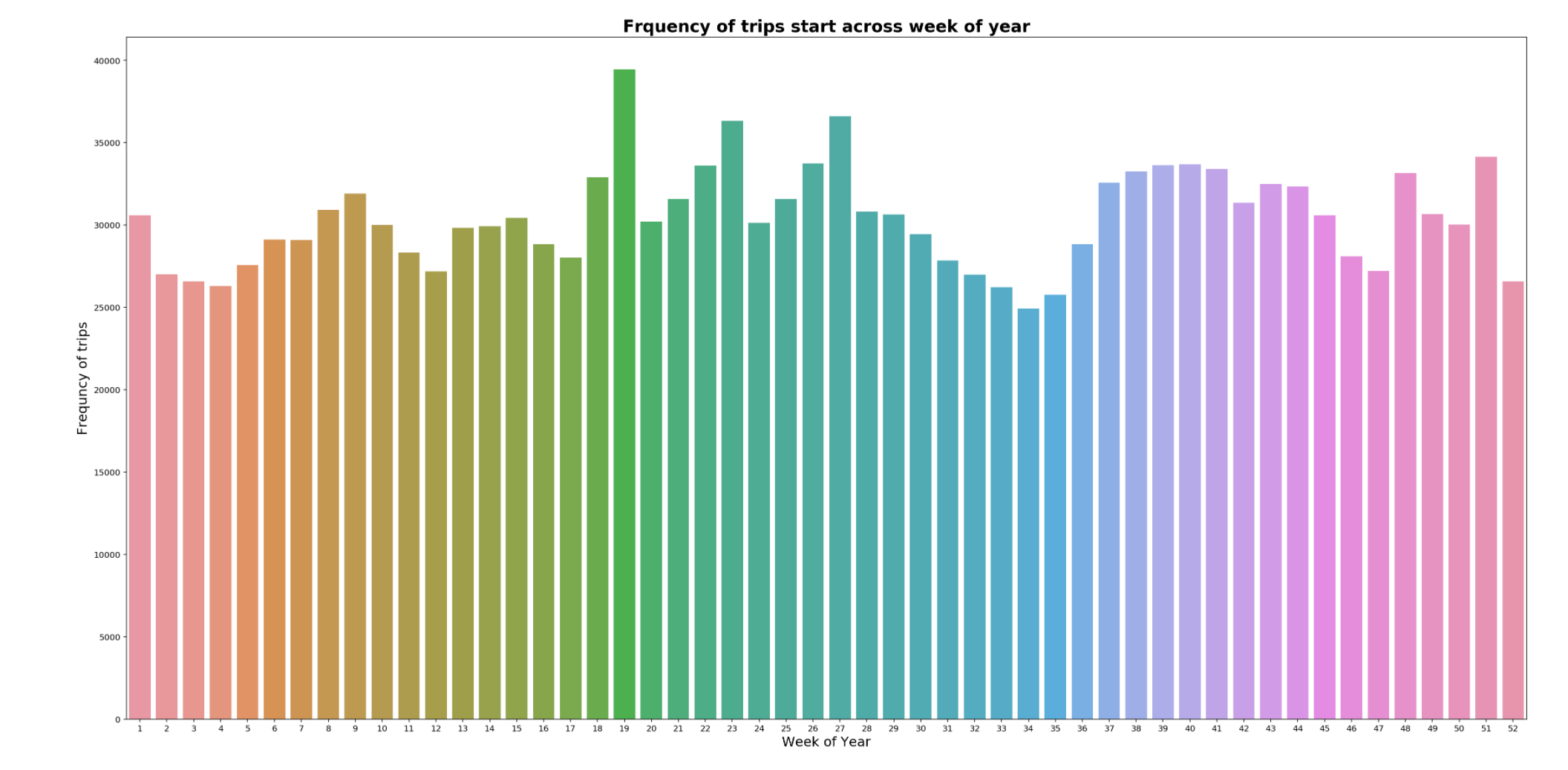
There appears to be a dip in taxi service in August 2013, lowest being in week 34, which is the summer school holidays in Porto. It appears that it could be either taxi drivers or customers going on holidays. The peak of taxi trips is in last week of April 2014, which is Spring in Porto.
49% of the trips are from taxi stands.
Train/Validation datasets
A validation set is created to determine the performance of model before using it to predict on our test set. As the given test set contains 320 truncated trips, we will split our training data into train and validation sets. The ratio chosen is train(99.9% - 1,580,976 trips) and validation(0.1% - 1,581 trips). In addition, the polyline coordinates of the validation set have to be truncated.
From research done by University of South Florida, five coordinates is required to conduct trajectory prediction analysis. Therefore, we shall use only the five and last five coordinates for our destination prediction.
Predictive Models
Regression - Tree Based Models
Regression tree based models chosen to predict the destination of our taxi trips. The choice for using regression trees are:
- Regression tree based models are able to predict multinomial outcome variables, which is ideal in our case as our outcome variables consist of two outputs (latitude and longitude)
- Decision boundaries of regression trees are rectilinear which is suitable for geospatial data as it is analogous drawing rectangles on a map to bound coordinates and using the centroid value as our predicted destination coordinates.
Therefore, both Decision Tree Regressor and Random Forest Regressor from sklearn packages will be used.
To adopt regression models the following steps are carried out:
- Conduct GridSearchCV for best minimum samples to split
- Use Decision Tree Regressor with best parameter found to train validate
- Use Random Forest Regressor with best parameter found above to train validate
The hyperparameter of the Decision Tree Regressor, minimum samples requried for a split, is chosen to grid search upon to determine how many coordinates should fall in a rectilinear boundary. Values 80, 100, 150, 250, 500 are chosen as split criteria.
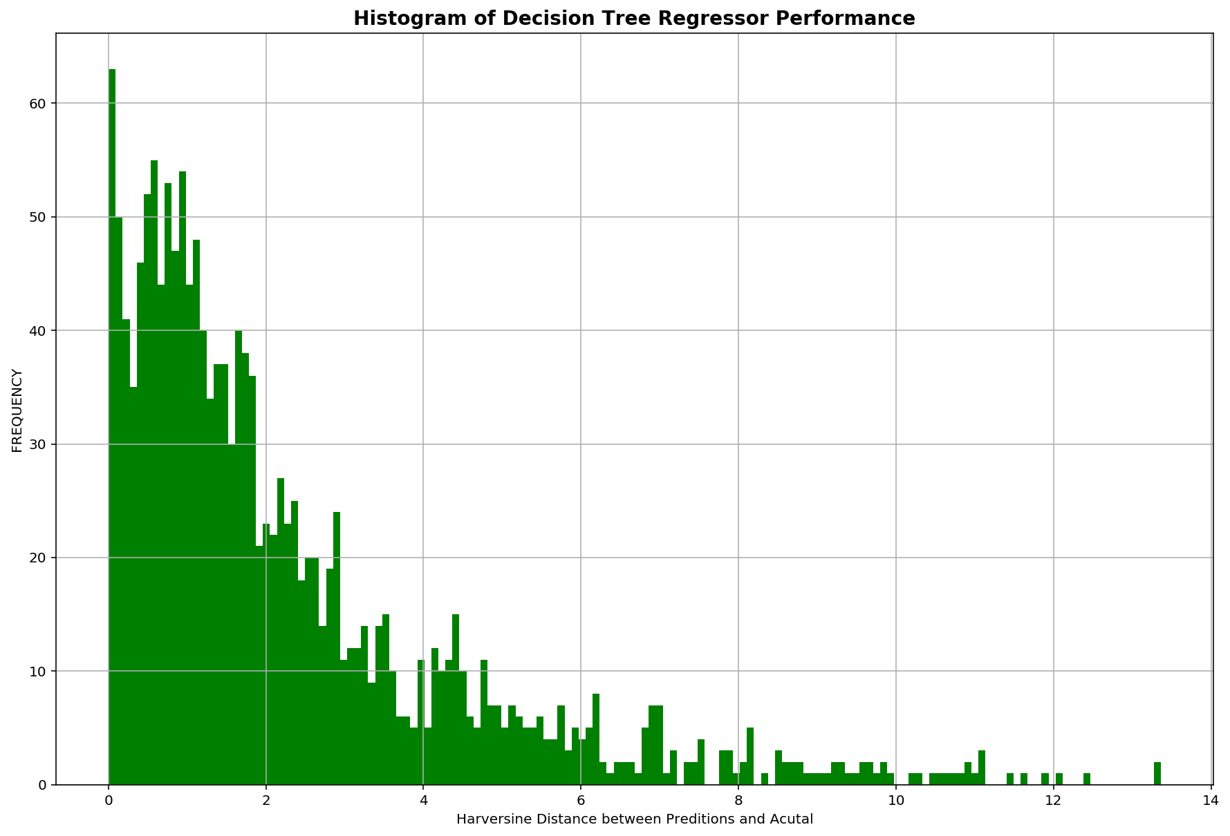
After gridsearch, best min samples split value is 100. Performance of the decision tree model is evaluated using the validation which resulted in an evaluation score of 2.26km.
As DecisionTreeRegressor decides splits based on a greedy algorithm, their accuracy performance might suffer as they tend to overfit the training set. In order to overcome this, we will use a RandomForestRegressor to help generalise the model through bagging techniques.
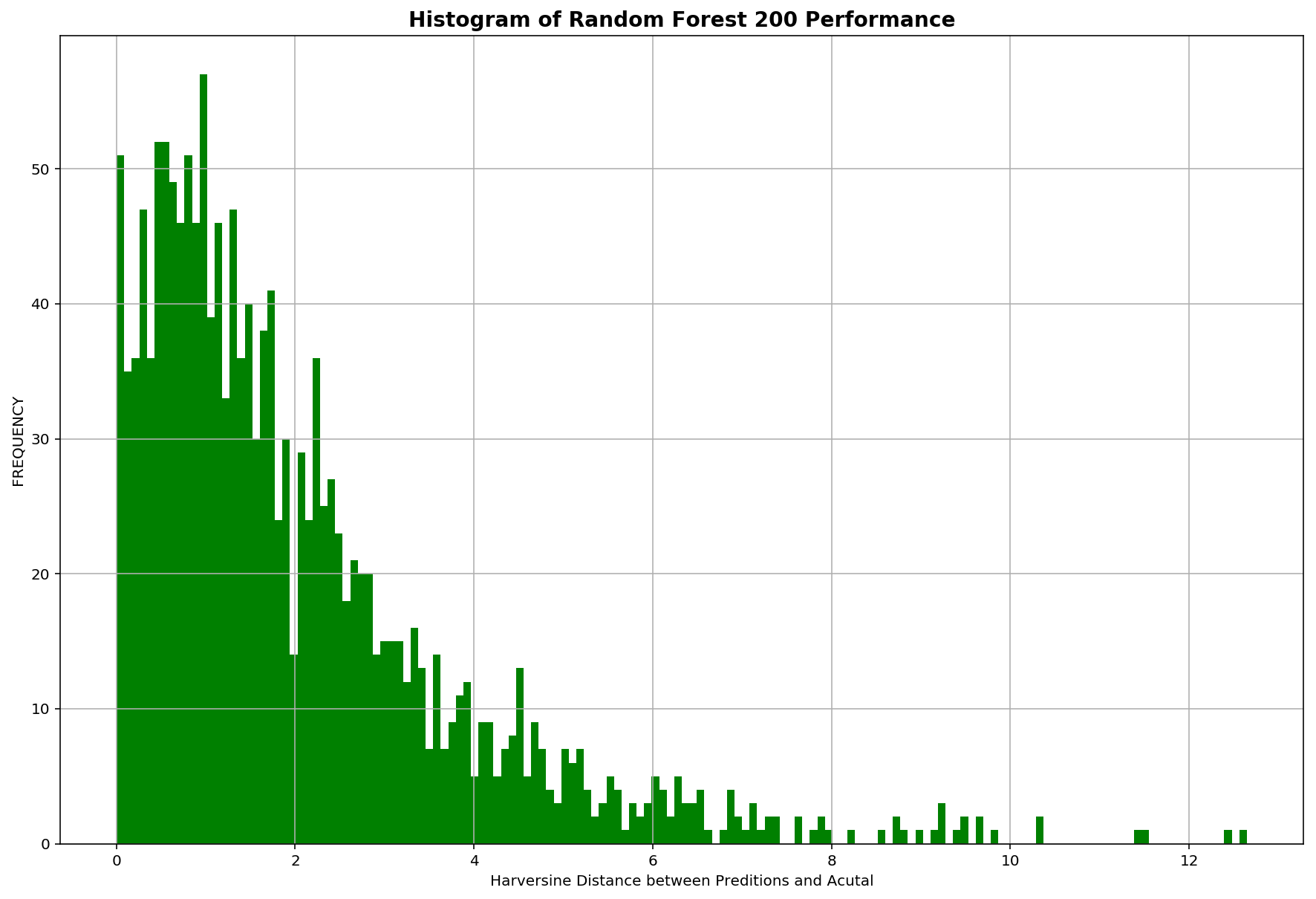
With the same DecisionTreeRegressor parameters, a RandomForestRegressor with 200 trees is used. Performance of the decision tree model is evaluated using the validation which resulted in an evaluation score of 2.03km. As expected, RandomForestRegressor improved our results by reducing the error in distance predicted over 200m.
The distribution of evaluation scores for both models:
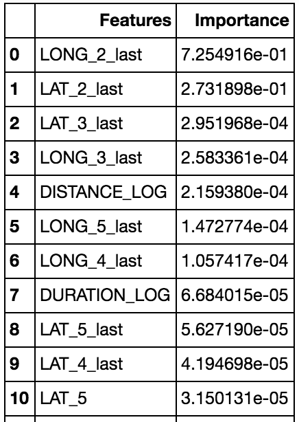
It is logical that the last subsequent coordinates before a trip ends is most predictive of a taxi ride’s destination and our model has also affirmed this as the 2nd and 3rd last coordinates are at the top for feature importance.
Classification – Neural Network
Besides using Tree Based Models, we shall use an Artificial Neural Network (ANN) to explore if we can increase the accuracy of destination predictions.
ANN is used as it takes all inputs into consideration - Each individual input connects to a neuron and when receiving input, change its internal state (i.e. the activation) according to that input and an activation function, and produce output depending on the input and the activation.
As a regression approach is used in for our Tree Based Model, a classification approach will be used in the ANN model.
To adopt an ANN the following steps are carried out:
- Form clusters of our destinations in our train set by rounding them to the fourth decimal place and geohashing them
- Split our train and val in to X (Predictor variables) and y (outcome variables) respectively
- Design and built our ANN model with Harversine distance as our custom loss function
- Fit X_train, y_train, X_val, y_val into our ANN to train it
- Plot Training and Validation Loss per epoch to determine how good our ANN is performing
- Chose the best model and use it to predict on our test set
To cluster our end destinations, a two step approach is taken:
- Extracting destinations coordinates in a pair. As latitudes and longitudes up to 4 decimals place have a precision of 11.132m, points along the same street with be effectively grouped together.
- After rounding, in order to further cluster coordinates into larger groups, coordinates are geohashed.
- Geohash encodes a geographic location into a short string of letters and digits. It is a hierarchical spatial data structure which subdivides space into buckets of grid shape, using hilbert space filling curves. Geohash package used
- Geohash precision of 17, using with base 4 (2bit) is chosen as it groups coordinates within (0.152703km x 0.152703km = 0.02km sq) together
- After encoding, geohashes are decoded to get the centroid coordinates representing each cluster
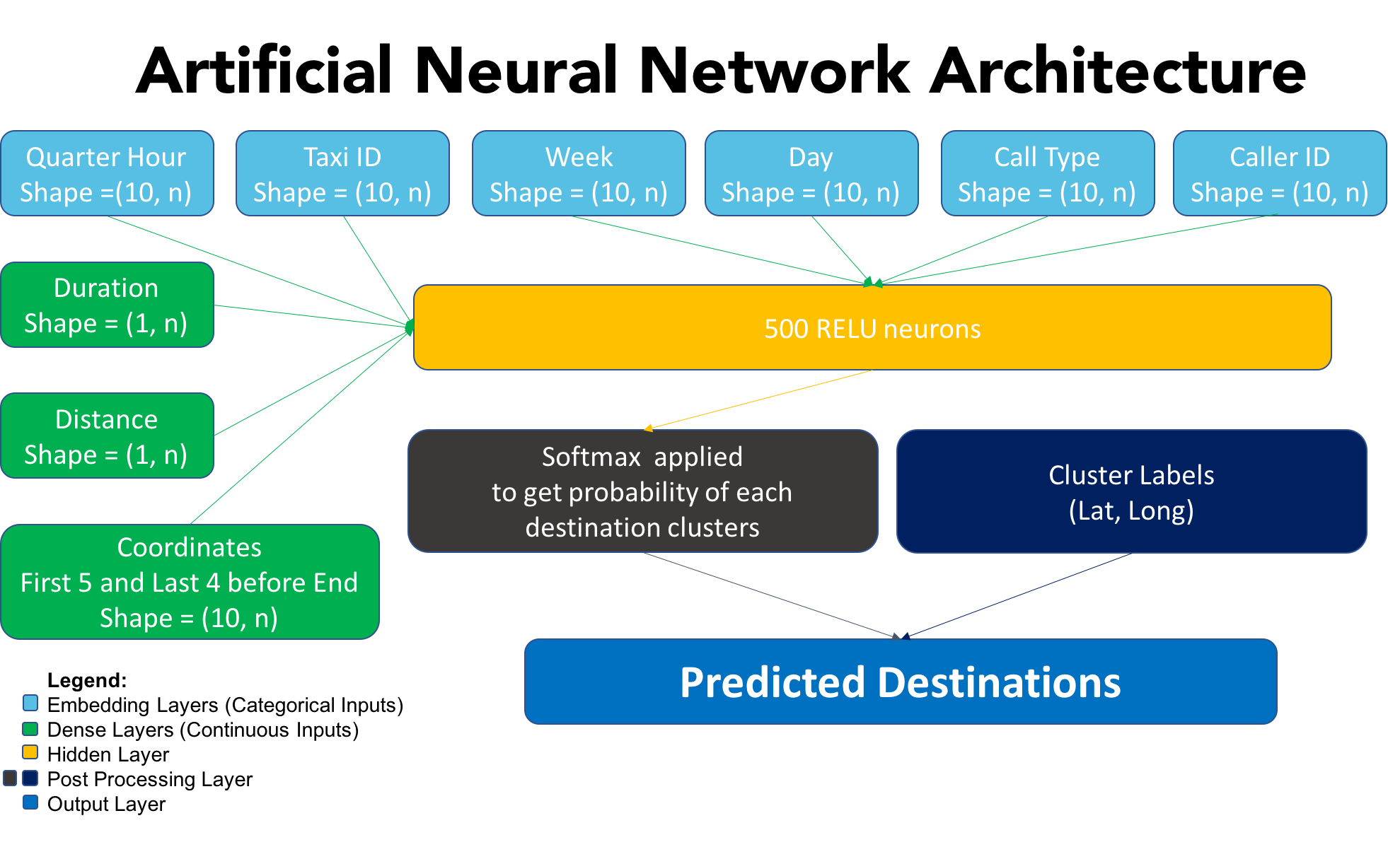
The architecture is fairly simple, a vanilla neural network. Keras with Tensorflow backend is used. Categorical features are inputted into an embedding layer (this is analogous to one hot encoding in other ML models). Continuous features are inutted into a dense layer (fully connected layer). One hidden layer with 500 neurons is used with Relu as the activation function. The output of the first layer is passed into a subsequent layer with a softmax activation to aggregate the probability of clusters, the highest probability will be chosen as the prediction in the output layer. The loss function used would be a custom loss function - the haversine distance. The ANN model will be striving to reduce the distance between the predicted and actual values of the validation set. In addition, the keras package do not take in pandas dataframes, therefore pre-processing of all inputs to numpy arrays (matrices and vectors) has to carried out.
After the building the framework of the model, the model is then trained on 50 epoch.
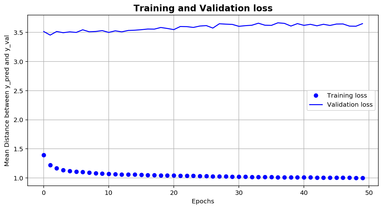
From the plot above, the training loss keeps decreasing, whereas the valiadation loss is rather consistent with minimal fluctuations. After epoch 20, the validation loss seems to have increased slightly, whereas the training continues to decrease. This shows that the model might be overfitting towards the training set.
Prediciting the test set
All three validated models created are then used to predict the test set with the predictions submitted and scored on Kaggle.
The results are:
- Random Forest Regressor
- Public score : 2.93471 Rank #100/381
- Private score : 2.84788 #244/381
- Artificial Neural Net
- Public Score: 3.02832 #115/381
- Private Score: 3.13960 #259/381
- Decision Tree Regressor
- Public score : 3.14168 #138/381
- Private score : 3.14442 #270/381
The Random Forest Regressor performed the best out of the three models.
Conclusion
Prediction of destinations up to 3km accuracy is possible with:
- Date & Time
- Location data in the form of coordinates
However, by adopting a classification model, due to the nature that the coordinates are extremely granular and there are places which the majority of the the public do not usually go, i.e farms in the outskirts of the city vs the city centre. The amount of points to form a cluster is extremely important to avoid a multivariate imbalance issue. However, it is extremely hard to determine the right amount of points required without domain expertise. Therefore, I strongly suggest using a regression model is more suited to predict destinations of trips.
Moving forward, the following approaches can be explored to improve the accuracy of our predictions:
- Use a regression ANN model to predict destinations
- Include more features, such as holiday, weather, driver and passenger information
- Use of deep learning models such as Sequence to Sequence Recursive Neural Nets and LSTMs, and other machine learning models, such as Hidden Markov Model and Karman filters to predict the path taken up to the destination
- Utilise Hadoop and Apache Spark architecture for scalability
Check out my full implementation of the project here. If you have and feedback or queries, I would love to hear them!:) Please leave a comment below or send me an email.

Derrick Lim
Data Science Practitioner | Travel & Hospitality Professional